T-distributed Stochastic Neighbor Embedding (t-SNE, van der Maaten and Hinton ‘08), is a dimensionality reduction technique commonly used for data visualization. In this post I’ll summarize how Stochastic Neighbor Embedding (SNE) works, which t-SNE is built off of. I’ll also implement SNE on the MNIST dataset. In a later post, I’ll summarize this wonderful post on distill.pub, and then implement t-SNE and test in on a couple of datasets.

Stochastic Neighbor Embedding

t-SNE shares its main idea with Stochastic Neighbor Embedding (SNE, Hinton and Roweis ‘02). SNE works with a mapping of the original high-dimensional points $x_i$ to points $y_i$ in a low-dimensional space. To evaluate how well the mapped points $y_i$ resemble the same structure as points $x_i$ , SNE does the following:

SNE first computes measures of similarity between the original points. For this, SNE uses conditional probabilities $p_{j \vert i} = \displaystyle\frac{\exp (- \vert\vert x_i - x_j \vert \vert^2 / 2\sigma^2_i)}{\sum_{k \neq i} \exp (- \vert\vert x_i - x_k \vert\vert^2 / 2\sigma^2_i)}$ to denote the probability of selecting point $x_j$ as a neighbor of $x_i$ . Note that these probabilities are drawn from the Gaussian distribution with $\mu = x_i, \sigma^2=\sigma^2_i$ . Assume that $\sigma_i$ is given for now – we’ll determine $\sigma_i$ from a parameter called perplexity, to be explained later.
Next, SNE computes the same conditional probabilities but on the low-dimensional points $y_i$ . We have that $q_{j \vert i} = \displaystyle\frac{\exp (- \vert\vert y_i - y_j \vert\vert^2)}{\sum_{k\neq i} \exp (-\vert\vert y_i - y_k \vert\vert^2)}$ .
If the pairwise similarity of points $y_i$ resemble that of the original points $x_i$ , then the conditional probability distributions $P_i = \{p_{j \vert i} \forall j\}$ and $Q_i = \{q_{j \vert i} \forall j\}$ will be similar as well. Therefore, as a measure of how well points $y_i$ model the similarities in points $x_i$ , we use the sum of the KL-divergences $\displaystyle\sum_i KL(P_i \vert\vert Q_i) = \sum_{i, j} p_{j \vert i}\log \frac{p_{j\vert i}}{q_{j \vert i}}$ .

To summarize, we create conditional probability distributions to model the pairwise similarity in both the low-dimensional points and high-dimensional points. When the two distributions are similar, the low-dimensional points $y_i$ appropriately models the similarity in points $x_i$ . As a result, we will optimize the KL-divergence between the two conditional probability distributions.

It’s worth noting that because KL-divergence is not symmetric, SNE also possesses asymmetric properties – KL-divergence assigns high cost when $x_i$ and $x_j$ are far but $y_i$ and $y_j$ are close, but it assigns a small cost for the opposite.

Deriving the SNE Update Rule

We have a cost function $C = \displaystyle\sum_i KL(P_i \vert\vert Q_i) = \sum_{i, j} p_{j \vert i}\log \frac{p_{j\vert i}}{q_{j \vert i}}$ . The goal of SNE is to find points $y_i$ which minimize this cost. To do this, we will compute the gradient $\displaystyle\frac{\partial C}{\partial y_i}$ . For the purpose of my own understanding, I worked out all the algebra for the gradient:

1) We have $\displaystyle\frac{\partial C}{\partial y_i} = \frac{\partial}{\partial y_i}\sum_{j, k} p_{k \vert j}\log \frac{p_{k\vert j}}{q_{k \vert j}}$ . 2) $\displaystyle\frac{\partial}{\partial y_i} p_{k \vert j}\log p_{k \vert j} = 0$ , because $p_{k\vert j}$ is independent from $y_i$ . As a result, we have

$$\displaystyle \frac{\partial C}{\partial y_i} = \frac{\partial}{\partial y_i}\sum_{j, k} (p_{k \vert j} \log \frac{1}{q_{k\vert j}}) = \sum_{j,k} (-\frac{p_{k \vert j}}{q_{k \vert j}}\frac{\partial q_{k \vert j}}{\partial y_i})$$.

3) This sum can be separated into two components:

$$\displaystyle\frac{\partial C}{\partial y_i} = \sum_j (-\frac{p_{j\vert i}}{q_{j\vert i}}\frac{\partial q_{j\vert i}}{\partial y_i} - \frac{p_{i\vert j}}{q_{i\vert j}}\frac{\partial q_{i\vert j}}{\partial y_i}) + \sum_{j, k \neq i} (-\frac{p_{k \vert j}}{q_{k \vert j}}\frac{\partial q_{k \vert j}}{\partial y_i})$$.

4) Now we evaluate the partial derivatives. For $q_{j\vert i}$ :

$$\displaystyle q_{j\vert i} = \frac{\exp (-\vert\vert y_i - y_j \vert\vert^2)}{\sum_{k\neq i} \exp (-\vert\vert y_i - y_k \vert\vert^2)} \\ \frac{\partial q_{j\vert i}}{\partial y_i} = \frac{\frac{\partial}{\partial y_i} \exp (-\vert\vert y_i - y_j \vert\vert^2)}{\sum_{k\neq i} \exp (-\vert\vert y_i - y_k \vert\vert^2)}-\frac{\exp (-\vert\vert y_i - y_j \vert\vert^2)\frac{\partial}{\partial y_i}(\sum_{k\neq i} \exp (-\vert\vert y_i - y_k \vert\vert^2))}{(\sum_{k\neq i} \exp (-\vert\vert y_i - y_k \vert\vert^2))^2} \\ = q_{j\vert i} 2(y_j - y_i) - q_{j\vert i}\frac{\frac{\partial}{\partial y_i} \sum_{k\neq i} \exp (-\vert\vert y_i - y_k \vert\vert^2))}{\sum_{k\neq i} \exp (-\vert\vert y_i - y_k \vert\vert^2))} \\ = q_{j\vert i} 2(y_j - y_i) - q_{j\vert i}\frac{\sum_{k\neq i} \exp(-\vert\vert y_i - y_k\vert\vert^2) 2(y_k - y_i)}{\sum_{k\neq i} \exp (-\vert\vert y_i - y_k \vert\vert^2))} \\ = q_{j\vert i} 2(y_j - y_i) - q_{j\vert i} \sum_{k\neq i} q_{k\vert i}2(y_k - y_i)$$.

5) For $q_{i\vert j}$ :

$$\displaystyle q_{i\vert j} = 1 - (\sum_{k\neq i, j} \exp (-\vert\vert y_j - y_k \vert\vert^2))\frac{1}{\sum_{k\neq i} \exp (-\vert\vert y_j - y_k \vert\vert^2)}\\ \displaystyle\frac{\partial q_{i\vert j}}{\partial y_i} = \frac{\partial q_{i\vert j}}{\partial y_i} = - (\sum_{k\neq i, j} \exp (-\vert\vert y_j - y_k \vert\vert^2)) \frac{-1}{(\sum_{k\neq j} \exp (-\vert\vert y_j - y_k \vert\vert^2))^2}\frac{\exp (-\vert\vert y_i - y_j\vert\vert^2)}{\partial y_i}\\ \displaystyle = \frac{1}{\sum_{k\neq j} \exp (-\vert\vert y_j - y_k \vert\vert^2)}\frac{\sum_{k\neq i, j} \exp (-\vert\vert y_j - y_k \vert\vert^2)}{\sum_{k\neq j} \exp (-\vert\vert y_j - y_k \vert\vert^2)} \exp (-\vert\vert y_j - y_i\vert\vert^2) 2(y_j - y_i) \\ = 2 q_{i\vert j} (1 - q_{i\vert j}) (y_j - y_i)$$.

5) For $q_{k\vert j}$ , $j, k \neq i$ :

$$\displaystyle q_{k\vert j} = \exp (-\vert\vert y_j - y_k\vert\vert^2)\frac{1}{\sum_{l\neq j} \exp (-\vert\vert y_j - y_l\vert\vert^2)} \\ \frac{\partial q_{k\vert j}}{\partial y_i} = \exp (-\vert\vert y_j - y_k\vert\vert^2)\frac{-1}{(\sum_{l\neq j} \exp (-\vert\vert y_j - y_l\vert\vert^2))^2}\frac{\partial \exp (-\vert\vert y_j - y_i\vert\vert^2)}{\partial y_i}\\ = \exp (-\vert\vert y_j - y_k\vert\vert^2)\frac{-1}{(\sum_{l\neq j} \exp (-\vert\vert y_j - y_l\vert\vert^2))^2}\exp (-\vert\vert y_j - y_i\vert\vert^2) 2(y_j - y_i) \\ = q_{k\vert j} \frac{-\exp (-\vert\vert y_i - y_j\vert\vert^2)}{\sum_{l\neq j}\exp (-\vert\vert y_j - y_l\vert\vert^2)}2(y_j - y_i)\\ = -2q_{k\vert j}q_{i\vert j}(y_j - y_i)$$

6) Reusing the sum from Part (3), we have

$$\begin{align*} \displaystyle\frac{\partial C}{\partial y_i} &= \sum_{j\neq i} (-\frac{p_{j\vert i}}{q_{j\vert i}}\frac{\partial q_{j\vert i}}{\partial y_i} - \frac{p_{i\vert j}}{q_{i\vert j}}\frac{\partial q_{i\vert j}}{\partial y_i}) + \sum_{j, k \neq i} (-\frac{p_{k \vert j}}{q_{k \vert j}}\frac{\partial q_{k \vert j}}{\partial y_i}) \\ &= \sum_{j\neq i} (-2p_{j\vert i} ((y_j - y_i) - \sum_{k\neq i} q_{k\vert i} (y_k - y_i)) - 2p_{i\vert j}(1 - q_{i\vert j})(y_j - y_i)) + \sum_{j, k\neq i} (2p_{k \vert j}q_{i\vert j}(y_j - y_i)) \\ &= -2\sum_{j\neq i} (y_j - y_i)(p_{j\vert i} + p_{i \vert j}(1 - q_{i\vert j})) + 2\sum_{j, k\neq i}p_{j\vert i}q_{k\vert i}(y_k - y_i) + \sum_{j, k\neq i} 2p_{k\vert j}q_{i\vert j} (y_j - y_i).\end{align*}$$

Taking advantage of the facts that $\sum_{j\neq i} p_{j\vert i} = 1$ and $\sum_{k\neq i} p_{k\vert j} = 1 - p_{i\vert j}$ , we have

$$\begin{align*} \frac{\partial C}{\partial y_i} &= -2\sum_{j\neq i} (y_j - y_i)(p_{j\vert i} + p_{i \vert j}(1 - q_{i\vert j})) + 2\sum_{k\neq i}q_{k\vert i}(y_k - y_i) + \sum_{j\neq i} 2(1 - p_{i \vert j})q_{i\vert j} (y_j - y_i)\\ &= 2\sum_{j\neq i} (y_i - y_j)(p_{j\vert i} + p_{i\vert j}(1 - q_{i\vert j}) - q_{j\vert i} - (1 - p_{i\vert j})q_{i\vert j}) \\ &= 2\sum_{j\neq i} (y_i - y_j)(p_{j\vert i} + p_{i\vert j} - q_{i\vert j} - q_{j\vert i}).\end{align*}$$

Perplexity

Hinton and Roweis (in the original SNE paper) introduce perplexity as a means of determining the values of $\sigma_i$ . As a result, perplexity specifies to what degree points $x_1, \ldots, x_n$ are considered the ‘neighbors’ for some point $x_i$ . It does so as follows:

For a fixed value of $\sigma_i$ , we have a corresponding distribution $P_i = \{p_{1\vert i}, p_{2\vert i}, \ldots, p_{n\vert i}\}$ .
Consider the Shannon Entropy of $P_i$ . That is, $H(P_i) = -\sum_j p_{j\vert i} \log_2 p_{j\vert i}$ .
When $\sigma_i$ is very small, the closest point to $x_i$ dominates the distribution, and $H(P_i) \approx 0$ . As $\sigma_i$ increases, the probabilities of all points become closer to each other and the Shannon Entropy increases. Perplexity determines our choice of $\sigma_i$ by making us select $Perp = 2^{H(P_i)}$ . Because $H(P_i)$ is an increasing function on $\sigma_i$ , there exists a unique solution for $\sigma_i$ for a given value of perplexity, which can be found using binary search.

Miscellaneous

Hinton and Roweis initialize the algorithm by randomly sampling $y_i$ from an isotropic Gaussian distribution. Also, momentum is used in the gradient descent algorithm for better performance. From the original paper:

$$\mathcal{Y}^{(t)} = \mathcal{Y}^{(t-1)} - \eta\displaystyle\frac{\partial C}{\partial \mathcal{Y}} + \alpha (t) (\mathcal{Y}^{(t - 1)} - \mathcal{Y}^{(t-2)}).$$

Implementation on MNIST

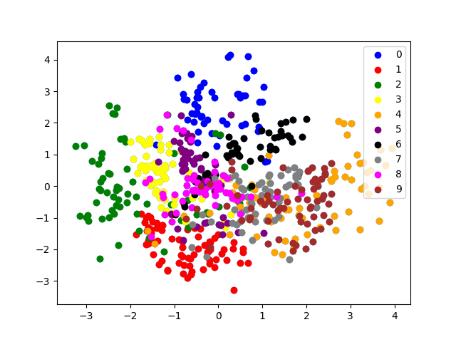
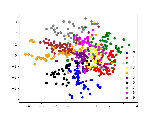
My implementation of SNE can be found here. To test my implementation, I ran it on the MNIST dataset (600 points, perplexity 20, 1000 iters). We get some pretty colorful graphs (these are for two separate runs of SNE):

It seems that SNE is somewhat effective at grouping images with the same labels together. In addition, classes which look similar are close together: the ‘4’ cluster is close to the ‘9’ cluster in both runs, as is the ‘3’ cluster and ‘8’ cluster. On the other hand, classes such as ‘2’ and ‘4’ which are very not-alike seem to be far apart.