Relearning Variational Inference

Next Post »

The other day, I realized that there’s a lot of content covered in MIT’s machine learning classes (6.867, 9.520) that I still don’t understand thoroughly, despite having taken these classes. So, this will be the first post in a hopefully long series where I take notes on materials I review.

Please be aware that a lot of the content covered in this post is taken from here.

The Problem

We want to construct a generative model which can deal with latent variables. What does this mean?

A generative model is a model which, given data, tries to learn the probabilistic distribution from which the data is generated. For example, a model that tries to learn the parameters $\mu, \sigma$ of a Gaussian distribution from data would be a generative model. Other examples of generative models include Hidden Markov Models or Latent Dirichlet Allocation.

On the other hand, discriminative models, such as a linear classifier, attempt to directly solve problems such as classification or prediction without learning the data distribution. In a supervised learning setting with data points $(X, Y)$, generative models can be thought of as learning the distribution $p(X, Y)$, while discriminative models learn $p(Y \vert X)$.

Latent variables, as Wikipedia explains, are “variables which that are not directly observed but rather inferred (through a mathematical model) from other variables that are observed (directly measured).” For example, consider the Gaussian mixture model below:

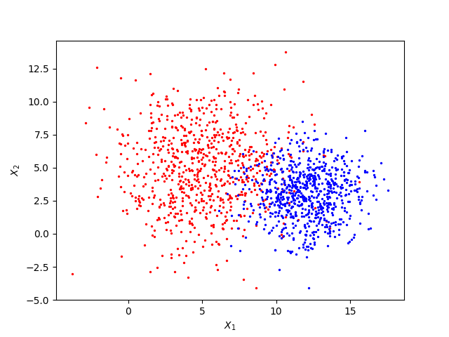
Here, the distribution of points is drawn from Gaussian 1 with $\mu = [5, 5]$ and $\sigma_1 = 3, \sigma_2 = 3$ with probability $0.5$, and from Gaussian 2 with $\mu = [12, 3]$ and $\sigma_1 = 2, \sigma_2 = 2$ with the remaining $0.5$ probability. In this example, the only two observed variables are the dimensions of the figure, $X_1$ and $X_2$. On the other hand, the $\mu, \sigma_1$, and $\sigma_2$ variables of each Gaussian are all latent variables. Although we can’t observe these parameters directly from the figure, they affect the distribution and we can infer them from the figure to some extent. Also note that the probability of a point being drawn from either Gaussian, in this case $(0.5, 0.5)$, is also a latent variable.

Circling back to our original problem statement, we want to construct a “model which learns the distribution of data” that can deal with “variables which we can’t observe directly, but affect the distribution and can be inferred.” For the remainder of this post, we will use the conventional notation $x_{1:n}$ to denote observed variables, and $z_{1:m}$ to denote latent variables.

Computing the Posterior

Let $\alpha$ denote the set of hyperparameters which we manually specify to determine the conditions from which the latent variables $z_{1:m}$ are generated. We’re interested in the posterior distribution:

$$p(z \vert x, \alpha) = \displaystyle\frac{p(z, x \vert \alpha)}{\int_z p(z, x \vert \alpha)}$$

The posterior distribution is useful because it’s essentially is a formalization what we want: given a set of observations, we want to learn and make inferences on the latent variables. By learning these latent variables, we’d be able to construct our desired generative model and learn the distribution from which $x_{1:n}$ is generated from.

Unfortunately, the posterior isn’t directly computable for a lot of distributions. Consider the following (Bayesian Mixture of Gaussians), taken from here:

1. Generate $\mu_1, \mu_2$ from $\mathcal{N}(0, \tau^2)$.

2. For $i = 1\ldots n$:

   a. Generate $z_i$ from $\pi = \{p(z=1) = 0.5, p(z=2) = 0.5\}$.

   b. Generate $x_i$ from $\mathcal{N}(\mu_{z_i}, \sigma^2)$.

In this example, we have the hyperparameters $\alpha = \{\tau, \pi, \sigma\}$. Our latent variables consist of $\mu_1, \mu_2$, and $z_{1:n}$. This is pretty similar to the mixture of Gaussians that we had previously – we just specified the distribution from which $\mu$ is generated, and fixed $\sigma$.

We have that $\displaystyle p(z, x, \mu \vert \alpha) = \prod^K_{k=1} p(\mu_k) \prod^n_{i=1} p(z_i) p(x_i \vert z_i, \mu)$. Equivalently, this equals

$$p(z, x, \mu \vert \alpha) = 0.5^n p(\mu_1) p(\mu_2) \prod^n_{i=1} p(x_i \vert z_i, \mu)$$

Consider the denominator of the posterior:

$$\int_{z, \mu} p(z, x, \mu \vert \alpha) = \int_{\mu_1, \mu_2} \sum_{z_{1:n} \in \{1, 2\}^n} 0.5^n p(\mu_1) p(\mu_2) \prod^n_{i=1} p(x_i \vert z_i, \mu)$$

This expression is not easy to evaluate. We can try to move the summation inside of the product:

$$0.5^n \int_{\mu_1, \mu_2} p(\mu_1) p(\mu_2) \prod^n_{i=1} \sum_{z_i \in \{1, 2\}} p(x_i \vert z_i, \mu)$$>

The $\displaystyle \prod^n_{i=1} \sum_{z_i \in \{1, 2\}} p(x_i \vert z_i, \mu)$ term is a product of $n$ sums of Gaussian probabilities $\displaystyle\frac{1}{\sqrt{2\pi\sigma^2}}e^{-\frac{(x_i-\mu)^2}{2\sigma^2}}$, and as far as I know there’s no reasonable way to simplify the inside expression of the integral into a closed-form expression. If we try multiplying out the inner product, we’ll get $2^n$ individual terms, which isn’t computationally viable. We can also try moving the summation outside:

$$0.5^n \sum_{z_{1:n}\in \{1, 2\}^n} \int_{\mu_1, \mu_2} p(\mu_1, \mu_2) \prod^n_{i=1} p(x_i\vert z_i, \mu)$$

Now the inside of the integral is computable, but we again have the problem of $2^n$ individual terms. So, we conclude that directly evaluating the exact posterior distribution is computationally intractable.

Variational Inference

Now here is the part where variational inference comes in. We resign ourselves to the fact that we can’t directly compute the posterior $p(z\vert x, \alpha)$, and instead select a family of distributions

$$q(z_{1:m} \vert v)$$,

with variational parameters $v$. The goal of variational inference is to determine $v$ such that $q(z_{1:m} \vert v)$ best approximates the original posterior $p(z \vert x, \alpha)$. Here you may have a couple of questions:

1. What would you select for a family of distributions $q$?
   • We’ll get to this later (see Mean-field variational inference).
2. What do you mean exactly by “best approximates”?
   • Yes, we need a formal measure of how well a distribution resembles another. This leads us to…

Kullback-Leibler Divergence

Frequently called KL-divergence, Kullback-Leibler divergence allows us to measure to what extent one probability distribution diverges from another:

$$KL(q \vert\vert p) = E_q [\log \displaystyle\frac{q(z)}{p(z \vert x)}] = \int_z q(z) \log \frac{q(z)}{p(z \vert x)}$$

Qualitatively, when optimizing for KL-divergence we just want to avoid cases when $q(z)$ is high and $p(z \vert x)$ is low. When $q(z)$ is low, the corresponding cost is also low since the cost is proportional to $q(z)$. When both $q(z)$ and $p(z \vert x)$ are high, then the corresponding cost is low as long as the two probabilities are of approximately the same magnitude.

It’s worth noting that KL-divergence is not symmetric: $KL(q \vert \vert p)$ does not necessarily equal $KL(p \vert \vert q)$. We purposely choose to use $KL(q \vert \vert p)$. We’ll later have to evaluate some expectations – since we’re able to compute $q(z)$ but not $p(z \vert x)$, it’ll be easier to work with $KL(q \vert \vert p)$, which takes expectations relative to $q(z)$. While there’s a form of variational inference which uses $KL(p \vert \vert q)$ called expectation propagation, I’m not too familiar with it and won’t be covered in this post.

Evidence Lower Bound

Turns out, KL-divergence is difficult to directly minimize because the posterior $p(z \vert x)$ still gives us trouble. We’ll use a nice trick called the evidence lower bound (ELBO) to get around this. From some nice math, we have:

$$\begin{align*} KL(q(z)||p(z|x)) &= E_q[\log \displaystyle\frac{q(z)}{p(z\vert x)}] \\ &= E_q[\log q(z)] - E_q[\log p(z \vert x)] \\ &= E_q[\log q(z)] - E_q[\log \displaystyle\frac{p(z, x)}{p(x)}] \\ &= -(E_q[\log p(z, x)] - E_q[\log q(z)]) + \log p(x) \end{align*}$$

The expression $E_q[\log p(z, x)] - E_q[\log q(z)]$ is the evidence lower bound. The $p(x)$ term does not depend on $q$ or the variational parameters $v$. As a result, maximizing the ELBO results in minimizing the KL-divergence. (If you’re interested, ELBO gets its name because it serves as a lower bound for $\log p(x)$. From this fact, it follows that KL-divergence is always non-negative.)

Summary

To recap, variational inference is a means for learning latent variables $z$ from the posterior distribution $p(z\vert x)$. Because the posterior is often difficult to compute, we resort to finding a similar distribution $q(z \vert v)$. By finding variational parameters $v$ which maximize the ELBO $E_q[\log p(z, x)] - E_q[\log q(z)]$, we also minimize KL-divergence and find the distribution $q(z \vert v)$ which best approximates the posterior.

In the next post, I’ll talk about mean-field variational inference, a specific instance of variational inference which places restrictions on $q$ and provides a way to maximize the ELBO.

References

1. https://www.cs.princeton.edu/courses/archive/fall11/cos597C/lectures/variational-inference-i.pdf.
2. https://www.quora.com/What-is-variational-inference. I liked Sam Wang’s summary: “In short, variational inference is akin to what happens at every presentation you’ve attended. Someone in the audience asks the presenter a very difficult answer which he/she can’t answer. The presenter conveniently reframes the question in an easier manner and gives an exact answer to that reformulated question rather than answering the original difficult question.”