Implementing Variational Inference

« Previous Post

Previously, I described the purpose and method of variational inference – a means to learn a distribution’s latent variables by finding a proxy distribution for the latent variables $q(z \vert v)$ and maximizing the Evidence Lower Bound (ELBO). Now, we’ll discuss how we can maximize the ELBO, and then implement what we’ve learned.

Mean Field Variational Inference

Mean Field Variational Inference is a specific instance of variational inference in which we choose a $q(z)$ that factorizes. That is,

$$q(z_{1:m}) = \prod^m_{i=1} q(z_i)$$

. In other words, each variable $z_i$ is independent. Now let’s use some math to simplify the ELBO. Recall:

$$ELBO = E_q[\log p(z, x)] - E_q[\log q(z)]$$

Expressing the joint probability $p(z, x)$ in terms of conditional probabilities,

$$\begin{align*} p(z, x) &= p(x)\prod^m_{i=1} p(z_i \vert z_{1:(i-1)}, x) \\ E_q[\log p(z, x)] &= E_q[\log p(x)\prod^m_{i=1} p(z_i \vert z_{1:(i-1)}, x)] \\ &= E_q[\log p(x) + \sum^m_{i=1} \log p(z_i \vert z_{1:(i-1)}, x)] \\ &= E_q[\log p(x)] + \sum^m_{i=1} E_q[\log p(z_i \vert z_{1:(i-1)}, x)] \end{align*}$$

Because $q(z)$ factorizes, we also have:

$$E_q[\log q(z)] = \sum^m_{i=1} E_q[\log q(z_i)]$$

Substituting both of these into the ELBO, we get

$$\begin{align*} ELBO &= E_q[\log p(z, x)] - E_q[\log q(z)] \\ &= E_q[\log p(x)] + \sum^m_{i=1} E_q[\log p(z_i \vert z_{1:(i-1)}, x)] - \sum^m_{i=1} E_q[\log q(z_i)] \\ &= E_q[\log p(x)] + \sum^m_{i=1} (E_q[\log p(z_i \vert z_{1:(i-1)})] - E_q[\log q(z_i)]) \end{align*}$$

Consider the ELBO as a function of $q(z_k)$. By rearranging how we express $p(z, x)$ in conditional probabilities, we can express the ELBO as

$$ELBO = E_q[\log p(z_k \vert z_{-k}, x)] - E_q[\log q(z_k)] + f(z_{-k}, x)$$

where $f(z_{-k}, x)$ does not depend on $z_k$ and is therefore a constant term. Now, given a fixed distribution for $q(z_{-k})$, we can derive the optimal $q^{\star}(z_k)$. Re-expressing the expectations, we note that

$$E_q[X] = \int q(z_k) E_{q_{-k}}[X] dz_k$$.

and therefore

$$ \begin{align*} ELBO &= \int q(z_k)E_{q_{-k}}[\log p(z_k \vert z_{-k}, x)] dz_k - \int q(z_k)E_{q_{-k}}[\log q(z_k)]dz_k + f(z_{-k}, x) \\ %\frac{\partial ELBO}{\partial q(z_k)} &= \int E_{q_{-k}}[\log p(z_k \vert z_{-k}, x)] dz_k - \int (E_{q_{-k}}[\log q(z_k)] + \frac{q(z_k)}{q(z_k)}) dz_k \\ %&= E_{q_{-k}}[\log p(z_k \vert z_{-k}, x)] - E_{q_{-k}}[\log q(z_k)] - 1 \\ %s&= E_{q_{-k}}[\log p(z_k \vert z_{-k}, x)] - q(z_k) - 1 \end{align*} $$.

When we consider that $\displaystyle\int q(z_k) dz_k = 1$, it turns out that we have a optimization problem which allows us to use the integral version of Lagrange multipliers. For those unfamiliar, details about using integral constraints can be found here and here, and may be covered in this blog at a later date. In essence, for some constant $\lambda$, the Lagrangian formulation leads to the condition

$$\begin{align*} q(z_k)E_{q_{-k}}[\log p(z_k \vert z_{-k}, x)] - q(z_k) E_{q_{-k}}[\log q(z_k)] &= \lambda q(z_k) \\ E_{q_{-k}}[\log p(z_k \vert z_{-k}, x)] - \log q(z_k) &= \lambda \\ q^{\star}(z_k) &= \exp (-\lambda + E_{q_{-k}}[\log p(z_k \vert z_{-k}, x)]) \\ \implies q^{\star}(z_k) & \propto \exp (E_{q_{-k}}[\log p(z_k \vert z_{-k}, x)]) \end{align*}$$

Because $p(z_k \vert z_{-k}, x) = \displaystyle\frac{p(z_k, z_{-k}, x)}{p(z_{-k}, x)}$ and $p(z_{-k}, x)$ is constant relative to $z_k$,

$$\begin{align*} p(z_k \vert z_{-k}, x) &\propto p(z, x) \\ \implies q^{\star}(z_k) &\propto \exp(E_{q_{-k}}[\log p(z, x)]) \end{align*}$$

Assuming that the normalized distrbution of $\exp(E_{q_{-k}}[\log p(z, x)])$ is computable, we now have a means for computing the optimal distribution of $q(z_k)$ when the other variables $z_{-k}$ are fixed. How do we use this?

Coordinate Ascent

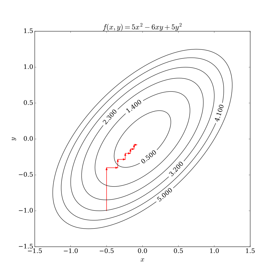
The coordinate ascent method allows us to converge to a local optimum. We iterate through each latent variable $z_i$, finding the optimum distribution when the other variables are fixed. An idea of how coordinate descent works on two parameters can be found here:

Implementation

Let’s revisit the Bayesian Mixture of Gaussians from the previous post:

1. Generate $\mu_1, \mu_2$ from $\mathcal{N}(0, \tau^2)$.
2. Uniformly randomly select $\pi_1$ from the interval $(0.25, 0.75)$.

3. For $i = 1\ldots n$:

   a. Generate $z_i$ from $\pi = \{p(z=1) = \pi_1, p(z=2) = 1 - \pi_1\}$.

   b. Generate $x_i$ from $\mathcal{N}(\mu_{z_i}, \sigma^2)$.

Under mean field variational inference, we choose a family $q(\mu_1, \mu_2, z_{1:n})$ where the distribution of $\mu_i$ is a Gaussian with parameters $\mathcal{N}(\widetilde{\mu_i}, \widetilde{\sigma_i}^2)$ and the distribution of every $z_i$ contains only two probabilities, $q(z_i = 1)$ and $q(z_i = 2)$. Each variable $\mu_1, \mu_2, z_{1:n}$ is independent, and therefore $q$ factorizes and requirement for mean field variational inference holds. From our previous derivations in the Mean Field Variational Inference section, we can obtain the following update rules for the variables in $q$:

$$q^{\star}[z_i = k] \propto \exp (\log \pi_k + x_i * \widetilde{\mu_k} - (\widetilde{\mu_k}^2 + \widetilde{\sigma_k}^2) / 2)$$

$$E[\mu_k] = \widetilde{\mu_k} = \frac{\sum^n_{i=1} q[z_i = k] x_i}{\sum^n_{i=1} q[z_i = k]} \\ Var[\mu_k] = \widetilde{\sigma_k} = \frac{1}{\sum^n_{i=1} q[z_i=k]}$$

Please note that we skipped all of the steps required to compute these two rules, which can be found in Section 8 of this. From here, it’s a simple matter of having a reasonable initialization of the variational parameters in $q$, followed by alternating through the update rules for $z_{1:n}, \mu_1, \mu_2$ for coordinate ascent.

An implementation of mean field variational inference on a Bayesian Mixture of Gaussians can be found here, which uses these two update rules.